Scratch Implementation of Logistic Regression
For the scratch implementation of logistic regression. We will be using Advertisement dataset which i took from Kaggle. Thanks to the Kaggle user fayomi for uploading dataset. Since, this topic is only focused on the Scratch implementation we will not talk much about the Data Preprocessing and Cleaning. Although there is not much to do in this dataset.
Basic Data Preprocessing :
In Data preprocessing we will 1st load and lean the dataset. Then we will split the cleaned dataset into train and test part. The Features of both train and test split should be normalized to make every feature contribute same amount of importance to model. Below is the code for the simple data preprocessing using sklearn.
After data preprocessing we can now move on to the scratch implementation to logistic regression but, before going into the code of scratch implementation we need the basic knowledge of Linear Regression and its equations.
What is Linear Regression?
Linear Regression is a supervised method that tries to find a relation between a continuous set of variables from any given dataset. Linear Regression can also be viewed as the single neuron feed forward neural network without the activation function. The equations to calculate the Linear Regression is:
y_hat = theta_0 + theta.T @ X                                  (1)
y_hat = theta.T @ X                                            (2)Where,
- .T represents the transpose of matrix theta and @ represents the dot product. - theta_0 and theta_1 are the weights and X is the features.- theta is the combination of theta_0 and theta_1. and X is the features with 1’s row array stacked on top of X.
    theta = [[theta_0],[theta_1]]
    X = [[1][X]]
To optimize the linear regression weights/ theta we will use MSE (Mean Square Error) and perform a gradient descent.
Now that, we have learned about the linear regression we can go on to logistic regressions. so,
What is logistic regression?
In a layman’s term Logistic regression can be understood as a upgrade to a linear regression. Upgrade to linear regression was addition of a Sigmoid Activation Function. The Sigmoid function takes the output of linear regression as input and outputs the value between 0 and 1.
sigmoid(z) = 1/( 1+e^(-z) )y_hat = sigmoid(Theta.T @ X) (3)
For optimizing the logistic regression weights/ theta different error function is used. We will be using entropy Binary Cross-Entropy / Log Loss and gradient descent.

Now we can continue with the coding part to implement the logistic regression. While implementing logistic regression we will directly convert our theory into code.
Coding of Logistic Regression:
Sigmoid Function : g(z)=1/(1+e^(−z))
Here, np.exp() represents the exponential (e)
Overall Cost Function:
In this code, np.sum() sums all the element of the matrix. for example:
if x is [[1,2][4,5]] matrix then np.sum(x) is equal to 12.
Calculate Cost: Calculating loss can be divided into two steps.
Step1: Predict output
- y_hat = sigmoid(theta.T @ X )
- y_hat = 1 / (1+e^(theta.T @ X))
Step2: Calculate Loss/Cost using target matrix (y) and predicted output matrix (y_hat)
- loss=J( y, y_hat)
In this code, np.dot() is used for matrix multiplication.
Calculate Gradient:
Calculating Gradient means measuring the change in weights with respect to the change in error. We can also think of a gradient as the slope of a loss function. To calculate gradient of weights/ Theta we will calculate the partial derivative of weights with respect to (W.R.T) overall loss.
Here is the final result of derivative of weights/ theta:
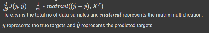
Implementing the derivative equation in code
Initializing theta or Weight matrix:
To define theta, we need to know the shape of a theta. Usually, the shape of the theta is always equal to size of (input_neuron, output_neuron) or (input_features, output_features).
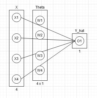
In case of logistic regression output feature is always 1 so we can define theta of shape (input_features,1)
Checking dimension of theta:
let y be the shape of (features_y, samples) = (1, samples) and X be the shape of (features_x, samples) = (4,samples). since we are predicting y from y_hat so y_hat should also be same as y in dimension. i.e y_hat = (1, samples)
using above rule (input_feature,output feature). dim of theta = (features_x, features_y) = (4,1)
y_hat=theta.T @ X
(1,samples) = (4,1).T @ (4,samples)
(1,samples) = (1,4) @ (4,samples)
(1,samples) = (1,samples) #After matrix multiplication
Code Implementation:
In code below np.zeros() is used to create the array with given dimension and fill it with zeros.
while implementation of this function. I have added +1 to input_feature because to handle bias / theta_0. *Look at logistic regression section*
Fit function:
Fit function to optimize our weight using gradient descent.
Training:
# Calling fit function to optimize the weightloss_plot, theta = fit(scaled_X_train, y_train, theta.T, lr=0.01, loop=2000)
Checking accuracy:
That’s it. we have covered scratch implementation of the logistic regression. You can find my notebook implementation in this link.
Thank you for reading.